
Using AI To Classify Website Screenshots
This article describes how the team at Urlbox built, trained and deployed a convolutional neural network (CNN) model that can classify screenshots of websites with an accuracy of 98.75%.
Written in Python, using the deep learning libraries of Tensorflow, given the URL of a website screenshot, it downloads the image, performs necessary preprocessing, and feeds this data to the model to classify the image. The result is a classification of the screenshot as either “successful” or “obscured”. The aim is to identify screenshots that have overlays, cookie banners, pop-ups, etc. that obscure the screenshot content and annoy Urlbox users.
 An example of a successful website screenshot
 The same website, but obscured (and classified as “obscured” by the model).
Early Attempts - Multi-Class Classification
Currently, we are only classifying screenshots as one of two categories: successful or obscured. However, early attempts included further categories, such as: broken and paywall.
Training the model on screenshots in these four categories proved an accuracy rate of 92% on the training set, but only 50% accuracy on the (unseen) validation set of screenshots. Which is not a sufficient accuracy to have any useful application.
However, removing the paywall screenshots from the training set (based on the assumption that paywall sites look relatively similar to successful sites), leaving the three categories of: successful, broken and obscured, resulted in 99% accuracy on training data and greater than 90% accuracy on (unseen) validation set of screenshots.
While having greater than 90% accuracy may seem sufficient for practical applications, we felt that due to the small number of instances in the broken category, it was best to remove this category entirely until we could collect a large enough number of broken screenshot instances before incorporating them back into the model.
Finally training the model on only successful and obscured screenshots resulted in an accuracy rate (on unseen data) of 98.75%.
Creating A Dataset of Website Screenshots
Despite there being some pre-existing datasets of classified websites screenshots, there were none that were suitable for the task at hand. So the dataset had to be created from scratch and the images manually classified.
Using a random sample of the websites from The Alexa Top Sites List, we used the URLs of the top ten most recent Google search results of these sites to then generate screenshots of those sites via the Urlbox API.
These were then manually classified as either successful or obscured.
While there are services that outsource the manual classification/labelling of images, such as AWS’s GroundTruth service in combination with AWS’s Mechanical Turk, to create large labelled datasets for deep learning projects such as this, getting set up with these services was deemed beyond the scope of this project. We wanted to build, train and deploy the model quickly without tying into a platform with which most of the team were unfamiliar. There are a few other ways to speed up the manual labelling step and deal with small (< 1,000 instances) datasets, without compromising the speed of the model’s development with the model’s final accuracy.
Firstly, simply scanning each downloaded screenshot and moving them to the correctly labelled directory, allowed over 100 screenshots for each category to be labelled within an hour or two.
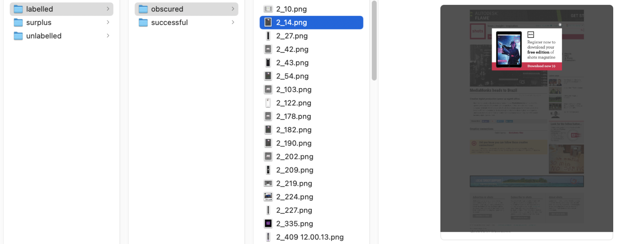 Example of screenshot manually labelled as “obscured”
Secondly, training the model, even on this small dataset, gave it some power of classification. Not enough that we would want to use the model in a production environment, but enough to assist with classifying further unseen data, which we can use to then increase the size of the dataset used for training the model.
We used the model trained on this small dataset to then classify unseen website screenshots. Clearly, there would be some misclassifications, but this step allowed us to rapidly classify a large number of screenshots using the partially trained model. These “first pass” classified screenshots were then rapidly scanned and any misclassified instances were removed or moved to the correct class/directory.
The model was then completely re-trained afresh using this larger dataset... that the model itself helped to create.
In addition to this, during training, we used a data augmentation step to create new, entirely synthetic versions of screenshots (using Keras’ ImageDataGenerator) , based on the existing screenshots, to further increase the size of the dataset used for training. Ultimately, all to increase the accuracy of the model on unseen data.
Choosing A Deep Learning Platform
There are a number of “off the shelf” deep learning platforms that aim to facilitate the whole deep learning pipeline or make it easier for those without experience in this area to create deep learning models.
When deciding which platform (if any) to use, one of the biggest factors in the decision should be: what platform/ ecosystem are the team currently using? We don’t want to burden the team with the extra cognitive load of having to learn a whole new ecosystem, just for a single application.
While one of the team has used AWS’ SageMaker platform previously for training and hosting deep learning models, the rest of the Urlbox team are more familiar with the Google Cloud Platform (GCP) ecosystem of services. So this gave us an opportunity to experiment with GCP’s VertexAI service.
Google Cloud Platform’s Vertex AI
This has a number of features that make training, deploying and hosting a deep learning model extremely easy.
Using VertexAI’s Image Classification Tutorial as a starting point, you will notice some extremely useful features, that you can take advantage of even if you don’t use the whole service. For example, during the data import process, I was warned that there was an error and not all the data was imported.
“Unable to import data due to errors… Warning: Annotation `successful` is deduped.”
It automagically detects and removes duplicate images during the import process. This is an extremely useful feature that can help clean your data.
Also, from the dashboard, you can quickly see exactly how many more instances you need of each class and it makes scanning the images (to make sure they are correctly labelled, etc) easier than on a local machine.
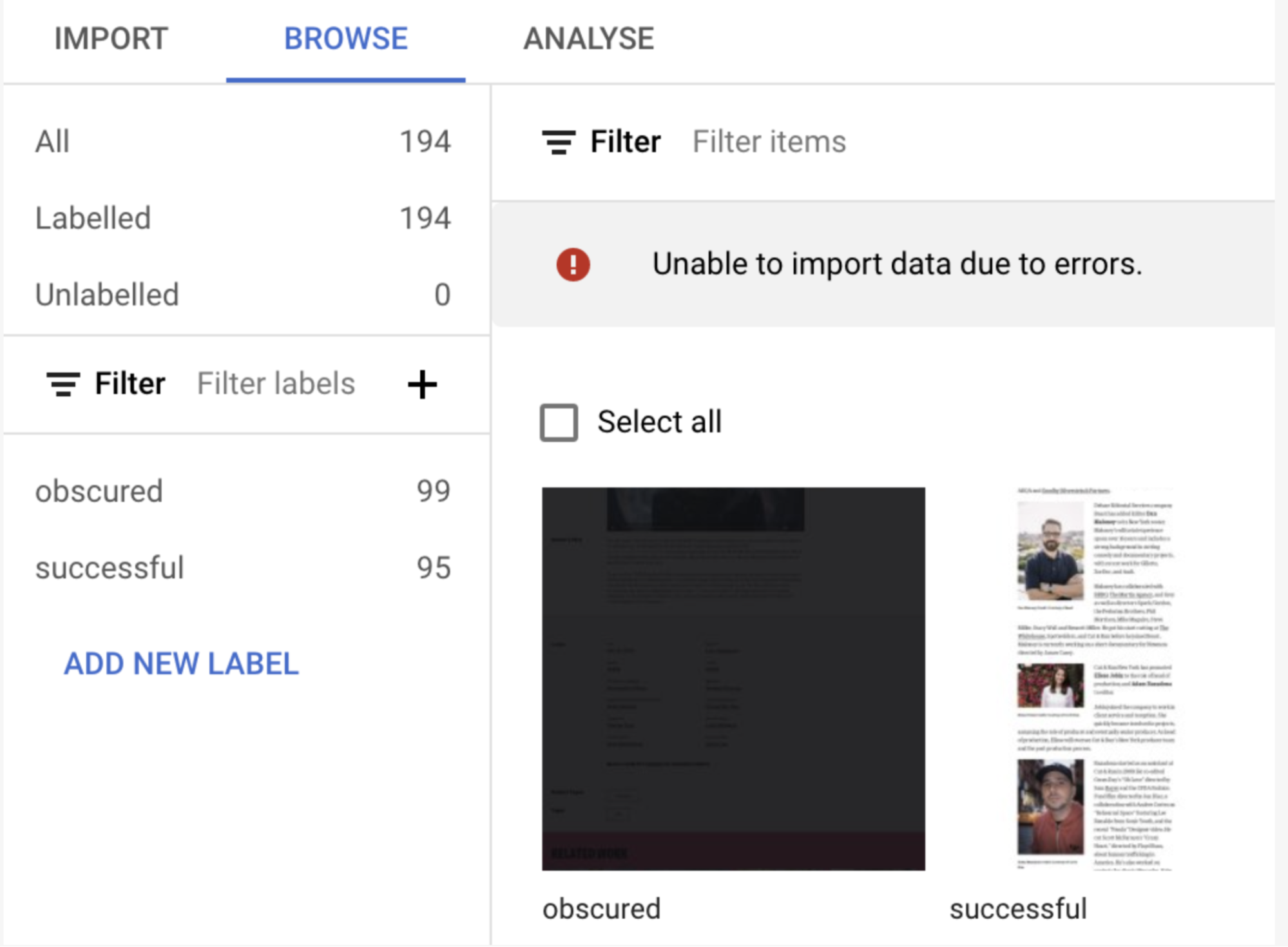 GCP’s VertexAI Dashboard - Showing number of instances in each class.
After correctly organising the dataset as required, the model was trained on a few hundred instances of both classes in approximately 30 minutes and reached an accuracy of 85%.
However, after an initial exploration, we choose not to commit to VertexAI. This was due to:
- The comparatively higher cost for training and hosting the model.
- The need to create an API wrapping the hosted model, before making a request. The VerexAI-hosted model endpoint isn’t a simple public endpoint as we had hoped. You still need to authenticate and then make a post request with the image as a base64 encoded string.
Instead, we created our own containerised Flask API to wrap the trained model and host it as a serverless application on GCP’s CloudRun (their managed serverless offering) service.
Training The Model
The model was trained by reading each image, and its associated label (successful, obscured) was determined by the name of the directory the image was in (/dataset/successful, dataset/obscured, etc) and then each image was preprocessed (resized, etc) and added to an array.
This array of images was then used to sample batches of images, which are fed to the model during the training process. The batch size, number of epochs and other hyperparameters can be tweaked to further improve accuracy, which I discuss later.
The architecture of the network (ie: number of layers, number of nodes in each layer, activation type, drop out rate, etc) was chosen based on the known successful rule of thumb for this type of network.
The code for this is below:
class BinaryCNN:
   @staticmethod
   def build(width, height, depth, classes):
      model = Sequential()
      inputShape = (height, width, depth)
      if K.image_data_format() == "channels\_first":
         inputShape = (depth, height, width)
      model = Sequential()
      model.add(Conv2D(32, (3, 3), input_shape=inputShape))
      model.add(Conv2D(64, (3, 3), activation="relu"))
      model.add(MaxPooling2D(pool_size=(2, 2)))
      model.add(Dropout(0.25))
      model.add(Conv2D(64, (3, 3), activation="relu"))
      model.add(MaxPooling2D(pool_size=(2, 2)))
      model.add(Dropout(0.25))
      model.add(Conv2D(128, (3, 3), activation="relu"))
      model.add(MaxPooling2D(pool_size=(2, 2)))
      model.add(Dropout(0.25))
      model.add(Flatten())
      model.add(Dense(64, activation="relu"))
      model.add(Dropout(0.5))
      model.add(Dense(1, activation="sigmoid"))
      return model
Moving from a multiclass classifier to a binary classifier required replacing the final, output layer of the network, which was a Softmax function (allowing multiclass classifications along with the associated probability of each classification) with a Sigmoid function (which is more suited to binary classification) (you can see this as the final layer in the above network architecture).
Adjusting the size of the images up to 224 x 224 pixels (from an original 80 x 80 pixels), increased the accuracy to greater than 90%. Further pre-processing of the images, by cropping them to 1024 x 1280 (to only train and classify on the top fold of the page) (before resizing to 224 x 224), and cleaning the data to reduce ambiguity in each class, finally increased accuracy to 98.75%
A sample of the training logs is shown below. Note the initial vs the final accuracy rate, of both the training data and the validation data (which is held back as unseen data to make sure the model is not overfitting on the seen, training data). We want to make sure that the accuracy rate and validation accuracy rate are similar. The validation accuracy rate tells us how accurate classifications will be on unseen data, which is what this application will be classifying in the real world. In this example, the model achieved an accuracy of 93.5% on the unseen data.
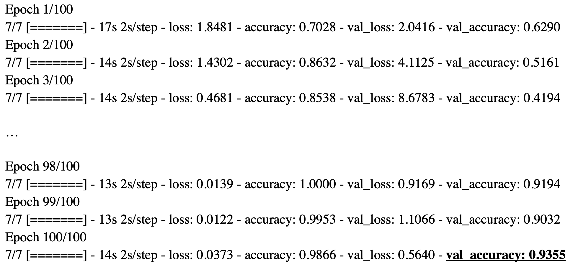 Example of the Training Logs
We use the EarlyStopping and ModelCheckpoint Keras callbacks to stop the training early and save the model once we have trained it to the highest accuracy on the validation (unseen) data.
Data Version Control
We use Data Version Control (DVC) to manage our dataset. It's too big to host on Github, so we host it on AWS’s S3 and then use DVC to pull it down to our local machine, to use when training. This allows other developers to continue with the project, using the data the model was trained on as a basis for further work. DVC can also be used to control the versioning of trained models, labels, etc.
Making a Classification Request
The trained model is wrapped up in a simple Flask API, which on start up loads the model from disk, then per request: downloads the image from its URL, performs required preprocessing and feeds the image to the model to make a classification.
A post request is made with a JSON body such as:
{
  "image_url": "https://some_example_screenshot_url.png"
}
And the response is the simply the classification of the screenshot, either “successful” or “obscured”:
{
  "classification": "obscured",
  "probability": 0.08571445941925049
}
Further Work To Increase Accuracy & Speed of Classification
We can use Keras’ autotuning of hyperparameters to randomly adjust the number of nodes, drop out rate, etc, of the inner layers of the network during training, finding the network hierarchy that results in the highest accuracy rate.
To reduce complexity to a minimum, the model was trained locally on a CPU, then wrapped in a Flask API and deployed to GCP’s CloudRun. However it could be retrained, and deployed, on a GPU, which has been shown to significantly reduce both training and inference/classification time (possibly up to 10x improvement). This should mean we reduce the time to classify screenshots to significantly under 1 second per classification.
